MTBF
Calculation
I
offer reliable MTBF-calculations for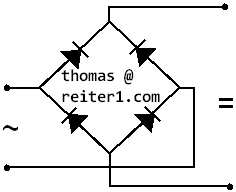
- electronics as well as for
mechanics
- according to many recognized
standards
- also for cases for which no
standard exists
You
will get a formal MTBF report describing the assumptions, the
calculation approach, and the results on system level and piece part
level, and, on any level in-between you need. If you have special
requests, just let me know and I will include it in the report
accordingly.
Here is a sample MTBF
report with dot and comma in US notation. If you prefer it vice
versa, your MTBF
report will be in international notation. This sample is for
electronics only. A mechanical (or mixed) MTBF report would be more
elaborate with respect to data sources & assumptions.
| Up
|
1. General Remarks
about MTBF / MTTF Calculation
|
Down
|
This is the MTBF calculation
page. If you need to know MTBF for your equipment, you're absolutely
right here. MTBF figures are needed, for example,
for functional safety projects and for maintenance planning.
The difference between MTBF and MTTF is negligible in most cases, and
very often it is just a matter of definition or convention. If you need
to know the difference, just go to the MTBF
page. From now on we will use the term MTBF only.
You are probably an R&D manager, or a development engineer, and you
probably just happen to face some MTBF related
issue, for example:
- the project specification has an MTBF requirement.
- This is quite likely for electronic equipment.
- your customer is asking for an MTBF figure
- your marketing department has heard about MTBF and wants to have
it
There are many reasons why MTBF
calculation has become an issue for you. Some are just nice to have, but many are real, for example:
- Someone needs MTBF just for marketing purposes. Then the only
thing that matters is the MTBF figure, which then should be as high as
possible. This would happen occasionally for electronic equipment.
- MTBF is needed for downstream calculations like
- expected maintenance / repair frequency and cost
- expected spares cost
- # of required onsite spares needed in order to meet reliability
/ productivity / etc. requirements
- functional safety:
safe failure fraction, probability of dangerous failure per hour for preferably electronics.
In 9 out of 10 cases when it comes to MTBF, we're talking about
electronics, for which several recognized MTBF calculation standards
exist. For mechanical equipment however, no such standards exist. We
will discuss electronics first.
Up
|
2. MTBF
Calculation for Electronics
|
Down
|
MTBF calculation for electronic equipment is usually performed with a
recognized MTBF calculation standard. Most of the information needed is
naturally given in bill of materials (BOMs). There are no specific
requirements concerning BOM content and
quality. The same BOM you would give to your assembler will be
fine.
Minimum information needed for
MTBF calculation
- BOMs
- Calculation standard.
- Environmental condition(s)
- For example: Ground mobile, ground benign
controlled, airborne inhabited cargo, naval unsheltered, ...
- Ambient temperature range
- For example from -40�C to +85�C in steps
of 5�C
- Temperature rise during operation (relevant for electronics, less relevant for mechanics.
- Keep this as simple as possible. In most
cases, the same (average) delta T for all piece parts would be fine.
In some cases, assigning individual dT for hot spots may be necessary.
If components of the system are exposed to different environments /
temperature(s), then, of course, components may be assigned
individual dT.
From
the above information I will be able to obtain reliable MTBF
figures on PCB level and on overall system level. On piece part level,
however, this approach will leave some or even many part type specific
questions unanswered, therefore producing many uncertainties on piece
part level. But fortunately this is only seldom an issue because,
generally speaking, many uncertainties tend to cancel each other out.
As mentioned above, this approach is the de facto industry standard,
and it is an interesting fact that the MTBF analyst doesn't need
electrical schematics, the BOM only is just fine.
This does not mean that electrical schematics don't have useful
information for MTBF calculation (in fact they have quite a lot), but
it means that BOMs alone contain sufficient information for reliable
MTBF figures on PCB and system level (but not on piece part
level). This will become clearer if you read further.
Optional information for MTBF calculation
If MTBF figures on PCB and
system level are not sufficient, and you also need reliable figures on
piece part level, then the following information will be needed
additionally. Please note that this
approach will probably be more costly, and you probably would need it
only for functional safety, military or aviation equipment (if at all).
- Individual dT for functional groups or even for every single
piece part.
- This would have substantial effect on piece part MTBF, but only
small effect on PCB and higher level MTBF.
- Useful / necessary only if there are big differences in dT
among piece parts or among functional groups.
- Before getting tangled up in these details, consider limiting
individual treatment to a small number of piece parts, for
example hot spots, and assigning average dT for all other piece parts.
- individual Stress levels (% of rating) for every single piece
part.
- The minimum approach described further above would use 50%
stress
(voltage, power , current, depending on which applies) for all piece
parts.
- Assigning individual stress levels would have substantial
effect on piece part MTBF, but only small effect on PCB and higher
level MTBF.
- Useful / necessary only if there are big differences in %
stress among piece parts.
- Before going this way,
- consider limiting
individual % stress treatment to a small number of piece
parts, and assigning average % stress (not necessarily 50%) for
all other piece parts, and,
- Before you start to
find out all % stress values on your own, asking me for
advice first would safe you a lot of unnecessary work!
Up
|
3. MTBF Calculation
for Mechanics
|
Down |
In contrast to electronics, there are no MTBF calculation standards
available for mechanical equipment. Nevertheless there is an increasing
demand for MTBF for mechanical equipment.
Field failure data, laboratory test data, and comparison with
similar equipment may be eligible data sources for MTBF calculation. If
asked, customers would often say that their field failure data is
useless, and
comparison with similar equipment won't work because of
technological difference. But
practical experience shows that the
reality is almost always more favorable than customers would expect.
For example, it often turns out that the field failure data is not so
useless
as it seems, or there is more information available than expected (e.g.
from other departments), or the technological difference is less MTBF
relevant than expected.
But even if customers were right with
their judgment, it would still not spoil these data sources, because
they may still be used as anchor points for (then seemingly more
uncertain) MTBF estimations, which are often called "engineering
judgment". But this would not be a pity at all, if communicated
honestly, since most MTBF calculations are uncertain anyway, even when
performed with a recognized MTBF calculation standard. The fact that no
MTBF
calculation standard is available for mechanical equipment doesn't add
much additional uncertainty, but it rather makes the inherent
uncertainty transparent. Finally, MTBF calculation is not only about
math,
statistics and engineering, but there is also a marketing aspect. For
example, when the MTBF of the predecessor was 100.000 h, then the MTBF
of the current item
should not be less, should it? The VP marketing will
probably have a say here.
What most engineers must learn about mechanical MTBF is the fact that probably a reasonable guess (often called engineering judgment) may be a valid data source, because it is
very often the only possible way. Engineers must learn to make valid
guesses.
In my career I was able to guide many customers to valid MTBF
judgments, which they were confident to defend and to communicate
to their customers.
Some readers may point to NPRD 1995, 2011 and 2016, which are
publicly available failure rate catalogs (not calculation standards)
for mechanical
components. However, despite being a kind of "holy grail" in
aviation and other industries, these catalogs often raise more
questions than they would answer. Picking
the right data set is often just like gambling. For example, if you
need to have a certain MTBF figure not less than one million hours, you
will probably find a satisfactory data set.
Up
|
4. MTBF Calculation
based on BOMs
|
Down
|
While MTBF is more intuitive, failure rates are easier to handle:
Failure rates can be just summed up in order to obtain a sum of failure
rates, but summing up MTBF would give apparently
nonsensical results.
As already mentioned further above,
MTBF calculation for electronic equipment usually means that a
recognized MTBF calculation standard is used. Most of the information
needed is
naturally given in bills of material (BOMs).
MTBF calculation standards can
be conceived as sets of mathematical formulas where each electronic
piece
part type (resistor, capacitor, ...) has its own dedicated formula.
For example, the formula for ceramic capacitors produces the failure
rate for a ceramic capacitor under certain (electric and environmental)
conditions. To give an idea, the following overly simplified example
may help:
Failure rate of a metal film resistor = power rating [W] x relative
power stress [%] / temperature [�C].
Below list describes the steps of
MTBF calculation based on BOMs.
I can assist you on any of these
steps:
- Chose the MTBF calculation standard.
- Define global parameters, e.g.
ambient temperature and environment.
- Your design engineer, maintenance technician, or the
requirements specification may provide this information.
- Identify all local
parameters for every piece part and calculate all piece part failure
rates.
- That's my job.
Each piece part type has its own specific set of parameters,
for example, capacitance for capacitors, # of transistors for linear
ICs, diode type (schottky, suppressor, general-purpose, ...)
- Sum
up all piece part failure rates, calculate MTBF = reciprocal of the sum
of
piece part failure rates, and create the MTBF report .
- That's my job, too.
The report will contain (among many other information) failure rate
and/or MTBF figures on PCB and system level for a range of temperatures
(e.g. from -40�C to +85�C in steps of 5�C), and on piece
part level for one selected
temperature. If you need more, just let me know.
MTBF
figures on PCB and system level may differ substantially depending
on the MTBF calculation standard, all other factors being
equal. A difference of factor of 3 on PCB level is quite normal, and
even factor 10 is possible.
The reason is that these standards have been established under
different circumstances and with different goals. More information on
this can be found at the bottom of the MTBF page.
On piece part level, the difference may
be even worse for specific parts, where factor 100 or even higher
may certainly happen from time to time. But this is irrelevant as long as you are
interested only in PCB level and system level MTBF.
Only in rare cases would MTBF figures on
piece part
level considered necessary, for
example in functional safety. Then,
step 3. (local parameters) in the above list becomes more
work-intensive because someone must identify stress levels and
temperatures for all piece parts. The good news is that I can show you
how to get this done efficiently.
But, again, provided that there is no
strong reason against it, I recommend that MTBF
calculations be performed with average
stress and temperature figures for every piece part.
Why do average temperature and stress figures on
piece part level still produce reliable MTBF figures on PCB and system
level? There are two reasons:
- One reason is just a statistical effect: If many independent
uncertainties with two possible directions (too low / too high) are
summed up, the result will not be a high, but rather a small
uncertainty, probably even smaller than the highest single
uncertainty.
This is just a simplified description of the so-called central limit
theorem, which belongs to the foundations of general statistics.
- The other reason comes from the MTBF calculation standards
themselves.
As
mentioned above, MTBF calculation standards are basically sets of
mathematical formulas, whose parameters
have been derived from comprehensive
field failure data. Nevertheless, each standard has at least a few part
types for which only limited field failure data was available,
therefore resulting in rather
coarse formulas that wouldn't take into account parameters that
otherwise would be considered important, for example temperature and
stress. The point is that these formulas tend to produce
rather high failure rates, and therefore these part types tend to
affect the PCB and system MTBF disproportionably.
Up
|
5. Calculating MTBF from Field
Failure Data correctly
|
Down |
This paragraph applies for laboratory
test
data, too.
Calculating MTBF from field or laboratory
data just by dividing the cumulative operating hours by the number of
fails seems intuitive, but unfortunately this is wrong. Even worse, it
would produce
optimistic figures, which can be dangerous if communicated to
customers.
Attentive
readers may suspect that dividing by the # of fails cannot be
correct for the simple fact that it doesn't work for
zero failures. This is even more interesting because zero failures
data sets are encountered quite often, in particular when the
cumulative operating hours is smaller than the (unknown) MTBF, or a
test is too short to produce a failure.
The actual reason however is that it ignores the random
character of failures, and instead implicitly assumes the failures
somehow to occur according to a (predictable) timetable. The fact that
failures (should) occur randomly is explained in depth on the MTBF page. The reason why
results become optimistic is more difficult to grasp, and maybe the
following example may help a bit:
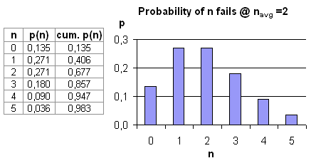 Suppose
the real MTBF was 500 h. Then the average outcome of a 1.000 hour test
would be 2 failures. Due to statistical variation however, the outcome
of a specific test may be 0, 1, 2, 3 or 4 failures, and even 5
and more cannot be ruled out, but if repeatedly tested, 2 failures
would be the average.
Now suppose you don't know the real MTBF, therefore you perform a 1.000
h test, and the outcome is 2 failures. What would be the best and
honest guess for the MTBF based on the given information, which is only
the test result? Here comes the poisson distribution into the game. The
picture shows the probability of n failures occurring in a 1.000 h test
provided that the average # of failures would be 2 (which equals MTBF =
500 h). Notice the following:
- The probability for up to 2 failures is
substantially higher than 0,5 (0,677).
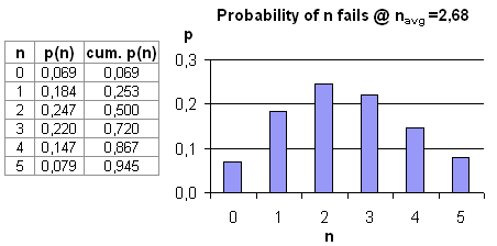 This
means: If 2 failures are encountered in a 1.000h test, the real MTBF
would be rather smaller than 500h, and therefore the best guess would
be some figure below 500 h. By playing with the poisson distribution,
we find that if the average # of failures was 2,68 instead of 2, the
probability of up to
2 failures in any specific selected test would be 0,5.
Therefore, if we don't know the real
MTBF figure, and our 1.000 h test produces 2 failures, the best guess
for the average number of failures within 1.000 h would be 2,68, which
transforms into the best guess MTBF = 1.000h / 2,68 = 373 h.
Note that randomness (failures occurring randomly) is the cause for
this. It's not a statistical issue, and in
particular it has nothing to do with statistical confidence.
Of course, an exact mathematical formula exists, so we don't need to
iteratively reverse-calculate MTBF with the Poisson.
More information on this can be found on the MTBF page.
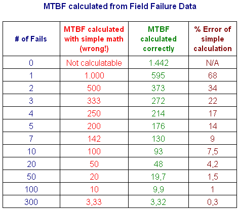
The table below shows calculated MTBF for a wider range of #
of failures. You may use it to estimate MTBF from field failure data or
from laboratory test data. In order to keep the table simple, the
underlying
cumulative operating time (or test duration) is always 1.000 h. MTBF
for any other cumulative operating time can be obtained by simple
linear conversion.
Please note:
- MTBF figures are rounded down, which is common practice in safety
engineering.
- MTBF
figures have 50% (upper and lower) statistical confidence.
- 50% statistical
confidence means the same as if no statistical
confidence was specified.
Up
|
6. The Foundation of
MTBF Calculation?
|
Down |
This paragraph aims to make the MTBF
calculation topic complete, from the perspective of someone who is
rather interested in how MTBF calculation works, than in the
theoretical background of MTBF (which is described in much more detail
on the MTBF page).
While MTBF is perceived as an intuitive metric, its underlying theory
is actually a bit complex in that sense that it addresses multiple
(seemingly uncorrelated) aspects at the same time. A good starting
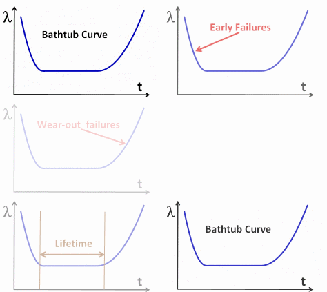
point is the so-called bathtub curve, in particular the middle part.
Constant
Failure Rate
 The
middle part of the bathtub curve has a constant failure rate. With
MTBF ~ 1/ failure rate, the MTBF is constant in the middle part.
Constant failure rate is not just a
simplification. The mathematical property
is
the same as the phenomenological property
If all failures occur randomly, then
no failure would occur systematically, therefore all failures would be
unpredictable, and finally no means would exist in order to prevent
failures.
This looks like an idealization at
first glance, but nevertheless does it perfectly describe companies
doing everything within their power in order to deliver flawless
products to customers. Such products would be free of foreseeable
failures, and all remaining failures that would still occur,
would be attributed to force majeure, because no means exists that
would prevent such failures.
Consequences
and Implications of Constant Failure Rate
- If failures occur only randomly,
preventive maintenance would have no effect, because prevention would
need predictability.
- Constant failure rate means that the
product doesn't age. Regardless of how long the product has been in
operation: as long as there is no failure, the product is always like
new. This is because due to future failures being unpredictable, past
failures wouldn't deliver any information for the prediction of future
failures. In other words, the failure history of a product doesn't tell
anything about future occurrences of failures. The only thing the
failure history does tell us is the failure rate.
More generally put: As long as products don't fail, they can be
considered as new products regardless of the time already spent in
operation.
- The constant failure rate property
turns out to be useful if field failure data is
limited. In this case, the constant failure rate property turns into a
helpful assumption because the model requires
less information than any other model with changing failure rate. In
many
cases, assuming constant failure rate is the only way at all to
establish a failure rate model.
The constant failure rate model needs only this information:
- Cumulative operating time of the
population of units,
- # of failures during that
time.
The constant failure rate model does NOT need:
- the
time points when the units failed,
- the
individual operating times of the units.
If you don't need time points and
individual operating times, the field failure information you once
considered useless suddenly becomes eligible for MTBF calculation.
Note that this is not a "trick", but
rather making existing information accessible.
Serial
Model
MTBF calculation generally assumes that
every piece part is equally important for the system function. Any
failure of whatever piece part would
cause a system failure. The picture below shows how
electrical schematics would look like in this model:
In
practice however, by far not every piece part failure would result in a
system failure, and even more, some failures wouldn't have any
noticeable effect at all. This is true even for "simple" (= neither
redundant nor otherwise fault tolerant) systems,
for example drift of some resistors and some capacitors, and even the
total
loss of some capacitors.
For such systems, the serial model turns out to be a bit
pessimistic. But this is no pity, and in safety context it
is even welcome.
However,
for redundant
or
otherwise fault tolerant systems, the serial model would give terribly
pessimistic MTBF because it would ignore the redundancy and fault
tolerance properties. For
such systems, MTBF (or failure rate) calculation would be applied only
on piece part and on functional group level, while for the system MTBF
more dedicated calculation methods like fault tree analysis, reliability block diagrams or markov analysis would be preferred.
MTBF figures on functional group
level would then serve as
quantitative input for these methods.




 Suppose
the real MTBF was 500 h. Then the average outcome of a 1.000 hour test
would be 2 failures. Due to statistical variation however, the outcome
of a specific test may be 0, 1, 2, 3 or 4 failures, and even 5
and more cannot be ruled out, but if repeatedly tested, 2 failures
would be the average.
  This
means: If 2 failures are encountered in a 1.000h test, the real MTBF
would be rather smaller than 500h, and therefore the best guess would
be some figure below 500 h. By playing with the poisson distribution,
we find that if the average # of failures was 2,68 instead of 2, the
probability of